
ROB-350 · Lesson 10 of 12 · 32 min
Planning for car-like and nonholonomic robots
A differential-drive robot can turn on the spot, so a path through free space in (x, y) is enough: the robot can stop, rotate to face the next segment and drive on. A car cannot. It can only move along its heading, and it can only change heading while moving, with a curvature limited by its steering. Forklifts, tugs pulling carts, tractors, ships and fixed-wing aircraft share the same kind of restriction. These nonholonomic constraints change planning fundamentally: a collision-free geometric path may be impossible to follow, and getting into a parking space may need a maneuver that goes backward and forward several times. This lesson explains what nonholonomic constraints are and why such robots can still reach every pose, introduces the Dubins and Reeds-Shepp curves that give shortest paths for car-like robots without obstacles, shows how these curves are used as steering functions inside the planners of lessons 5 and 7, and touches on trailers and differential flatness.
Nonholonomic constraints
For a robot moving in the plane with pose \( (x, y, \theta) \), the condition that it cannot slide sideways is
This constrains velocities, not positions, and it cannot be integrated into a relation among x, y and θ alone, which is what makes it nonholonomic. The robot therefore has three configuration variables but only two independent ways to move: forward along its heading and turning. Remarkably, it can still reach any pose, because combining the two motions generates the missing sideways one: drive forward while turning left, back up while turning right, and repeat, and the car shuffles sideways, as in parallel parking. In control theory this is the Lie bracket of the two motion directions, and Chow's theorem guarantees that when the brackets span all directions the system is controllable. For planning, the consequence is that every pose is reachable, but the path to a nearby pose may be long and complicated.
Worked problem
The bicycle model
A car-like robot follows the kinematic bicycle model \( \dot{x} = v\cos\theta,\ \dot{y} = v\sin\theta,\ \dot{\theta} = (v/L)\tan\delta \), with wheelbase L = 1.6 m and maximum steering angle 35°. What is its minimum turning radius, and how much road width does a U-turn need?
Show solution
- Minimum radius of the rear-axle path: \( R_{\min} = L/\tan\delta_{\max} = 1.6/\tan 35^{\circ} = 1.6/0.700 = 2.29 \) m.
- A U-turn with no reversing traces a semicircle of diameter \( 2R_{\min} = 4.57 \) m measured at the rear axle.
- The body is wider than a point: adding a vehicle width of, say, 1.0 m gives at least 5.6 m of road.
Answer: About 2.3 m minimum radius and roughly 5.6 m of road for a U-turn without reversing; a narrower road requires a three-point turn.
Dubins curves
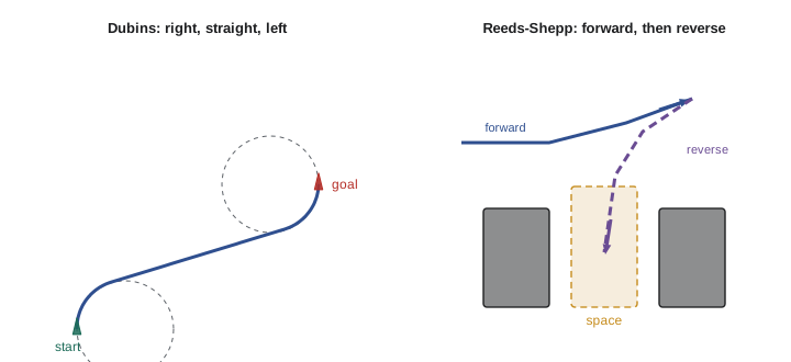
In 1957 Lester Dubins proved that for a vehicle that can only move forward at constant speed with curvature bounded by \( 1/R \), the shortest path between two poses in the absence of obstacles is always made of at most three segments, each either a circular arc of radius R turning left (L) or right (R), or a straight segment (S). Only six combinations can be optimal: LSL, RSR, LSR, RSL, RLR and LRL. To find the shortest Dubins path, compute the length of all six (some may not exist for a given pair of poses) and take the smallest. Each takes a few lines of trigonometry, so the whole computation runs in microseconds. Dubins paths are the right model for robots that cannot reverse, such as fixed-wing aircraft at constant altitude or boats, and they are the steering function in many kinodynamic sampling planners.
Worked problem
An LSL Dubins path
A robot with minimum turning radius R = 2 m starts at (0, 0) heading 90° (north) and must reach (10, 6) heading 90°. Compute the length of the LSL path, turning left at both ends.
Show solution
- Left-turn circle centers lie R to the left of each heading. Start: (0 − 2, 0) = (−2, 0). Goal: (10 − 2, 6) = (8, 6).
- For LSL the straight segment is parallel to the line joining the centers: from (−2, 0) to (8, 6), length \( \sqrt{100 + 36} = 11.66 \) m, direction \( \operatorname{atan2}(6, 10) = 30.96^{\circ} \).
- The first left turn takes the heading from 90° to 30.96°, but turning left increases heading, so it must go from 90° all the way round to \( 360^{\circ} + 30.96^{\circ} \): a turn of \( 300.96^{\circ} = 5.25 \) rad, arc length \( 2 \times 5.25 = 10.51 \) m.
- The second left turn takes 30.96° to 90°: \( 59.04^{\circ} = 1.03 \) rad, arc length 2.06 m.
- Total: \( 10.51 + 11.66 + 2.06 = 24.23 \) m.
Answer: About 24.2 m, mostly because the first turn nearly loops all the way round. The RSL candidate, an S-shaped path of about 12.6 m, is roughly half as long, which is why all six types are evaluated and the minimum taken.
import math
def mod2pi(a): return a % (2 * math.pi)
def dubins_lengths(x0, y0, t0, x1, y1, t1, R):
    """Lengths of the six Dubins words using the standard normalized formulas; None if infeasible."""
    dx, dy = x1 - x0, y1 - y0
    d = math.hypot(dx, dy) / R; th = math.atan2(dy, dx)
    a, b = mod2pi(t0 - th), mod2pi(t1 - th)
    sa, ca, sb, cb, cab = math.sin(a), math.cos(a), math.sin(b), math.cos(b), math.cos(a - b)
    out = {}
    p2 = 2 + d * d - 2 * cab + 2 * d * (sa - sb)                     # LSL
    out["LSL"] = None if p2 < 0 else (mod2pi(math.atan2(cb - ca, d + sa - sb) - a) + math.sqrt(p2) + mod2pi(b - math.atan2(cb - ca, d + sa - sb)))
    p2 = 2 + d * d - 2 * cab + 2 * d * (sb - sa)                     # RSR
    out["RSR"] = None if p2 < 0 else (mod2pi(a - math.atan2(ca - cb, d - sa + sb)) + math.sqrt(p2) + mod2pi(math.atan2(ca - cb, d - sa + sb) - b))
    p2 = -2 + d * d + 2 * cab + 2 * d * (sa + sb)                    # LSR
    if p2 < 0: out["LSR"] = None
    else:
        p = math.sqrt(p2); tmp = math.atan2(-ca - cb, d + sa + sb) - math.atan2(-2, p)
        out["LSR"] = mod2pi(tmp - a) + p + mod2pi(tmp - b)
    p2 = d * d - 2 + 2 * cab - 2 * d * (sa + sb)                     # RSL
    if p2 < 0: out["RSL"] = None
    else:
        p = math.sqrt(p2); tmp = math.atan2(ca + cb, d - sa - sb) - math.atan2(2, p)
        out["RSL"] = mod2pi(a - tmp) + p + mod2pi(b - tmp)
    t = (6 - d * d + 2 * cab + 2 * d * (sa - sb)) / 8                # RLR
    if abs(t) > 1: out["RLR"] = None
    else:
        p = mod2pi(2 * math.pi - math.acos(t)); tt = mod2pi(a - math.atan2(ca - cb, d - sa + sb) + p / 2)
        out["RLR"] = tt + p + mod2pi(a - b - tt + p)
    t = (6 - d * d + 2 * cab + 2 * d * (sb - sa)) / 8                # LRL
    if abs(t) > 1: out["LRL"] = None
    else:
        p = mod2pi(2 * math.pi - math.acos(t)); tt = mod2pi(-a + math.atan2(-ca + cb, d + sa - sb) + p / 2)
        out["LRL"] = tt + p + mod2pi(mod2pi(b) - a - tt + p)
    return {w: (None if v is None else v * R) for w, v in out.items()}
L = dubins_lengths(0, 0, math.radians(90), 10, 6, math.radians(90), 2.0)
for w, v in L.items():
    print(w, "infeasible" if v is None else "%.2f m" % v)
best = min((v, w) for w, v in L.items() if v is not None)
print("shortest word: %s, %.2f m (straight-line distance %.2f m)" % (best[1], best[0], math.hypot(10, 6)))LSL 24.23 m RSR 24.23 m LSR 36.23 m RSL 12.59 m RLR infeasible LRL infeasible shortest word: RSL, 12.59 m (straight-line distance 11.66 m)
Reeds-Shepp curves
Cars can reverse. In 1990 Reeds and Shepp extended Dubins' result to a vehicle that may drive forward or backward with bounded curvature. The shortest path then has at most five segments, with cusps where the direction changes, and belongs to one of 46 families (48 in the original count, two of which are redundant). Reeds-Shepp paths are never longer than Dubins paths between the same poses, and they are typically much shorter for nearby poses that differ mainly in position sideways or heading, where reversing helps, as in parallel parking. They are the obstacle-free distance used as a heuristic in Hybrid A* (lesson 5) and as the analytic expansion that completes its search, and they are available in OMPL as a state space for sampling planners. One subtlety: Reeds-Shepp paths minimize length, not the number of direction changes, so practical planners add a penalty for each cusp, since stopping and reversing take time and are less comfortable.
Worked problem
Why reversing helps
A car with R = 3 m is at (0, 0) heading east and must reach (0, 1.0) heading east, a 1 m sideways shift. Roughly how long is a forward-only Dubins path, and how does a Reeds-Shepp path compare?
Show solution
- Forward only, the car must leave, loop and come back: a typical Dubins solution here is two turns of almost a full circle combined, about 2πR ≈ 19 m, plus a little.
- With reversing, a sideways shift of 1 m is an S-shaped maneuver: turn left forward through a small angle, then turn right backward through the same angle (or vice versa), and straighten.
- Each arc needs an angle θ with \( 2R(1 - \cos\theta) = 1 \), giving \( \cos\theta = 1 - 1/6 = 0.833 \), \( \theta = 33.6^{\circ} = 0.586 \) rad; four such arcs (forward left, forward right, then repeated in reverse to return to the original x) total about \( 4 \times 3 \times 0.586 = 7.0 \) m.
Answer: Roughly 19 m forward-only against about 7 m with reversing. For small lateral corrections, reversing maneuvers are far shorter, which is why parking planners use Reeds-Shepp curves.
Using steering functions in planners
Dubins and Reeds-Shepp curves ignore obstacles, but they are exact steering functions: given two poses, they return the shortest feasible connection. Planners use them in three ways. As heuristics, their lengths are admissible lower bounds on the true cost, so they guide A* on lattices and in Hybrid A*. As local planners, they replace straight lines in PRM and RRT: to connect two samples, compute the curve between them and check it for collisions; OMPL's DubinsStateSpace and ReedsSheppStateSpace do this, letting RRT* and PRM* plan for car-like robots directly. And as final connections, they finish a search exactly at the goal pose, which grid search alone cannot do. For robots with more complex dynamics, such as a car at speed where tire forces matter, these geometric curves are replaced by trajectory optimization or motion primitives computed from the full model.
| Model | Allowed motion | Shortest path structure | Typical robots |
|---|---|---|---|
| Holonomic / omnidirectional | Any direction | Straight line | Mecanum-wheel platforms |
| Differential drive | Forward, backward, turn on the spot | Rotate, straight, rotate | Indoor mobile robots |
| Dubins | Forward only, bounded curvature | At most 3 segments, 6 words | Fixed-wing aircraft, boats |
| Reeds-Shepp | Forward and backward, bounded curvature | At most 5 segments, 46 families | Cars, forklifts, tugs |
| Car with continuous curvature | Curvature changes at bounded rate | Clothoid-based curves | Road vehicles at speed |
Trailers, curvature continuity and flatness
Real vehicles complicate the picture. Dubins and Reeds-Shepp paths switch instantly between straight lines and full-lock turns, which requires the steering wheel to jump; real steering changes at a finite rate, so planners for road vehicles use continuous-curvature paths built from clothoids (curves whose curvature changes linearly with length), which are slightly longer but drivable at speed. A tractor pulling one or more trailers adds a heading variable per trailer and a hitch-angle constraint, and reversing a trailer is unstable without feedback, as any driver knows. Lattice planners with primitives computed for the full articulated model are the usual answer, as in automated port and airport tugs. Finally, some nonholonomic systems are differentially flat: there exist flat outputs (for a car, the rear-axle position) such that the whole state and input can be computed from the output trajectory and its derivatives. For such systems, planning reduces to finding a smooth enough curve for the flat outputs, often with polynomials, and the steering and speed follow algebraically. Quadrotors are also flat, with position and yaw as outputs, which is why polynomial trajectory planning is standard for drones.
Worked problem
Steering from a flat output
For the bicycle model, curvature along the rear-axle path is \( \kappa = \tan\delta / L \). A planned path has curvature 0.25 m⁻¹ at some point, and L = 2.7 m. What steering angle is needed, and is it within a 32° limit?
Show solution
- \( \tan\delta = \kappa L = 0.25 \times 2.7 = 0.675 \).
- \( \delta = \arctan 0.675 = 34.0^{\circ} \).
- This exceeds the 32° limit.
Answer: About 34°, beyond the limit. The planner must keep curvature below \( \tan 32^{\circ}/2.7 = 0.231 \) m⁻¹, a radius of at least 4.3 m.
Common mistakes
MistakePlanning a car-like robot with a 2-D grid and expecting the controller to follow sharp corners
InsteadRespect the turning radius in planning with lattices, Hybrid A* or Dubins/Reeds-Shepp steering.
MistakeComputing only one Dubins word
InsteadEvaluate all six candidates and take the shortest.
MistakeUsing Dubins curves for a robot that can reverse
InsteadUse Reeds-Shepp curves; reversing maneuvers are often much shorter.
MistakeIgnoring the cost of direction changes
InsteadAdd a penalty per cusp so the planner avoids unnecessary shuffling.
MistakeSending full-lock instant steering changes to a fast vehicle
InsteadUse continuous-curvature paths at speed.
Summary and key terms
- Nonholonomic constraints restrict velocities, for example no sideways sliding, without restricting reachable positions.
- Combining forward motion and turning generates sideways motion, so car-like robots can reach every pose.
- The bicycle model gives the minimum turning radius from wheelbase and steering limit.
- Dubins paths, at most three arc or straight segments, are shortest for forward-only vehicles with bounded curvature.
- Reeds-Shepp paths add reversing, with at most five segments, and are much shorter for parking-like maneuvers.
- These curves serve as heuristics, local planners and exact final connections in grid and sampling planners.
- Trailers, continuous curvature and differential flatness extend planning to more realistic vehicles.
- Nonholonomic constraint
- A non-integrable constraint on velocities.
- Bicycle model
- A kinematic model of a car with one steered front wheel and one rear wheel.
- Minimum turning radius
- The tightest circle a vehicle can follow.
- Dubins path
- Shortest forward-only path with bounded curvature, of at most three segments.
- Reeds-Shepp path
- Shortest forward-and-backward path with bounded curvature.
- Cusp
- A point where the vehicle changes direction of travel.
- Steering function
- A method returning a feasible connection between two states.
- Clothoid
- A curve whose curvature changes linearly with arc length.
- Differential flatness
- A property letting all states and inputs be computed from flat outputs and their derivatives.
- Controllability
- The ability to reach any state with suitable inputs.
Practice problems
Work each problem on paper first, then reveal the answer to check.
Write the no-sideways-slip constraint.
Show answer
\( \dot{x}\sin\theta - \dot{y}\cos\theta = 0 \).
Minimum radius for L = 2.5 m and 30° steering?
Show answer
2.5 / tan 30° ≈ 4.33 m.
How many Dubins words can be optimal?
Show answer
Six.
What does S mean in a Dubins word?
Show answer
A straight segment.
Can a Reeds-Shepp path be longer than a Dubins path between the same poses?
Show answer
No.
Why add a cusp penalty?
Show answer
Direction changes cost time and comfort.
How does Hybrid A* use Reeds-Shepp curves?
Show answer
As a heuristic and as an analytic final connection.
What curve gives continuous curvature?
Show answer
A clothoid.
Curvature limit for L = 3 m, steering limit 30°?
Show answer
tan 30° / 3 ≈ 0.19 m⁻¹.
Name a flat output for a quadrotor.
Show answer
Its position and yaw.
Lesson quiz · 5 questions
Score 60% or more to complete this lesson.
Create a free account to save your progress, take quizzes and earn a certificate.