
ROB-350 · Lesson 3 of 12 · 28 min
Graph search I: breadth-first search and Dijkstra's algorithm
Once free space has been turned into a graph, whether a grid of cells, a visibility graph, a lattice of motion primitives or a roadmap of sampled configurations, planning becomes graph search: find a sequence of edges from the start node to a goal node, ideally one with the smallest total cost. Graph search is the workhorse of motion planning. It runs inside almost every mobile robot planner, inside the query phase of probabilistic roadmaps, and inside the high-level task planners that sequence robot actions. This lesson covers the uninformed searches, breadth-first search and Dijkstra's algorithm, which find shortest paths without any hint of where the goal lies. Lesson 4 adds heuristics that point the search toward the goal.
The algorithms here are the same ones met in CMPUT-204, but in robotics their details matter in specific ways: how the graph is generated (usually on demand rather than stored), what the edge costs mean, how ties are broken, and how the cost of the priority queue compares with the cost of checking whether an edge is collision-free. Understanding these practical points is what separates a planner that runs in milliseconds from one that runs in seconds.
Graphs for planning
A graph consists of nodes (vertices) and edges joining pairs of nodes, each edge with a non-negative cost. In a grid, each free cell is a node and edges join neighboring cells. With 4-connectivity, a cell connects to its four orthogonal neighbors at cost 1 (times the cell size); with 8-connectivity, it also connects to the four diagonal neighbors at cost \( \sqrt{2} \). Larger neighborhoods (16-connected) add knight-like moves and produce smoother paths at higher cost. In a roadmap, nodes are sampled configurations and edges are short collision-free motions between them. In a state lattice, nodes are discretized states and edges are precomputed motion primitives the robot can actually execute.
Planning graphs are often implicit: rather than building the whole graph and storing it, the planner generates a node's neighbors only when it needs them, checking each candidate edge for collisions at that moment. This matters because the full graph may be enormous, a 1000 by 1000 grid has a million nodes and eight million edges, while a search typically touches only a fraction of it. Implicit graphs also make it easy to change costs as the map changes.
| Graph | Nodes | Edges | Typical use |
|---|---|---|---|
| 4-connected grid | Free cells | Orthogonal neighbors, cost 1 | Simple, fast; staircase paths |
| 8-connected grid | Free cells | Plus diagonals, cost √2 | Most 2-D mobile robot planners |
| Visibility graph | Obstacle vertices, start, goal | Mutually visible pairs | Exact shortest paths in the plane |
| Probabilistic roadmap | Sampled free configurations | Short collision-free connections | Arms, multi-query planning |
| State lattice | Discretized states (x, y, θ) | Feasible motion primitives | Car-like robots |
Breadth-first search
Breadth-first search (BFS) explores the graph in layers: first every node one edge from the start, then every node two edges away, and so on. It keeps a first-in, first-out queue called the frontier or open list, and a record of which nodes have been reached and from where. When the goal is removed from the queue, the path is recovered by following the parent pointers back to the start. BFS finds the path with the fewest edges, which is the shortest path when every edge has the same cost, as on a 4-connected grid. Its running time is \( O(|V| + |E|) \), linear in the size of the graph, which makes it the fastest possible exhaustive search.
BFS is also the basis of the wavefront or brushfire algorithm used in many planners. Starting from the goal, assign each free cell its BFS distance; then, from any start, simply move to the neighbor with the smallest distance until the goal is reached. The resulting distance field is a navigation function with no local minima, so a robot can follow it from anywhere. Running the same flood from the obstacles instead gives each cell's distance to the nearest obstacle, which is the basis of clearance costs and of cost map inflation.
Worked problem
A wavefront by hand
On a 4-connected grid, a goal is at cell (0, 0) and a wall occupies cells (1, 0) and (1, 1). What is the wavefront value of cell (2, 0), and what path does a robot starting there follow?
Show solution
- Distance 0 at (0, 0). Distance 1: (0, 1). Distance 2: (0, 2). Distance 3: (1, 2).
- Distance 4: (2, 2). Distance 5: (2, 1). Distance 6: (2, 0).
- From (2, 0), step to the neighbor with value 5, then 4, and so on: (2, 1), (2, 2), (1, 2), (0, 2), (0, 1), (0, 0).
Answer: The value is 6, and the robot follows the descending values around the end of the wall. Each step reduces the value by one, so the robot can never get stuck.
Dijkstra's algorithm
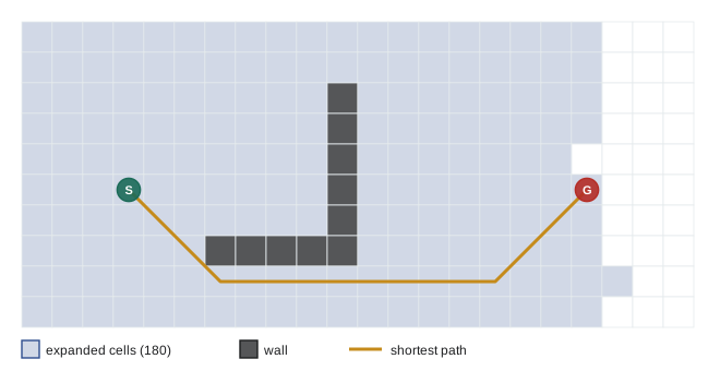
When edges have different costs, as with diagonal moves or with cost maps that penalize proximity to obstacles, BFS no longer finds the cheapest path. Dijkstra's algorithm, published by Edsger Dijkstra in 1959, generalizes it. It keeps for each node a tentative cost g, the cheapest known cost from the start, and a priority queue ordered by g. At each step it removes the node with the smallest g, which is then final, and relaxes its edges: for each neighbor, if reaching it through the current node is cheaper than its current g, the neighbor's g and parent are updated and it is placed in the queue. The algorithm stops when the goal is removed from the queue.
Dijkstra is correct because edge costs are non-negative: once a node has the smallest g in the queue, no later path can reach it more cheaply, since every remaining path costs at least as much before it even arrives. Negative edge costs break this argument, but planning costs are never negative. With a binary heap the running time is \( O((|V| + |E|) \log |V|) \). On an 8-connected grid where \( |E| \approx 8|V| \), this is nearly linear, and for a million-cell grid Dijkstra runs in well under a second in compiled code.
import heapq, math
grid = ["..........",
        "..........",
        "...####...",
        "......#...",
        ".S....#.G.",
        "......#...",
        "...####...",
        ".........."]
R, C = len(grid), len(grid[0])
start = goal = None
for r in range(R):
    for c in range(C):
        if grid[r][c] == "S": start = (r, c)
        if grid[r][c] == "G": goal = (r, c)
moves = [(dr, dc, math.hypot(dr, dc)) for dr in (-1, 0, 1) for dc in (-1, 0, 1) if dr or dc]
g = {start: 0.0}; parent = {start: None}; pq = [(0.0, start)]; expanded = 0
while pq:
    d, u = heapq.heappop(pq)
    if d > g[u]: continue                 # stale queue entry
    expanded += 1
    if u == goal: break
    for dr, dc, w in moves:
        v = (u[0] + dr, u[1] + dc)
        if 0 <= v[0] < R and 0 <= v[1] < C and grid[v[0]][v[1]] != "#":
            if d + w < g.get(v, math.inf):
                g[v] = d + w; parent[v] = u; heapq.heappush(pq, (g[v], v))
path = []; n = goal
while n: path.append(n); n = parent[n]
print("path cost: %.3f cells" % g[goal])
free = sum(ch != "#" for row in grid for ch in row)
print("path has %d cells; nodes expanded: %d of %d free" % (len(path), expanded, free))path cost: 10.657 cells path has 10 cells; nodes expanded: 67 of 69 free
Priority queues and implementation details
The priority queue dominates Dijkstra's cost, and its implementation matters. A binary heap is the usual choice. Most libraries do not support decreasing a key in place, so implementations push a new entry when a node's cost improves and skip outdated entries when they are popped, the 'lazy deletion' used in the code above. This costs a little memory but is simpler and often faster. When edge costs are small integers, a bucket queue (Dial's algorithm) gives constant-time operations. Tie-breaking also matters on grids, where many paths have equal cost: breaking ties in favor of nodes closer to the goal, or of the most recently inserted node, reduces the number of expansions and changes which of the equal-cost paths is returned.
Edge-cost design is where robotics enters. A pure distance cost gives the shortest path, which hugs walls. Adding a cost that grows near obstacles, read from an inflated cost map, trades a little length for clearance. Adding a cost for each change of direction gives straighter paths. Unknown cells can be treated as free (optimistic planning, useful for exploration) or as expensive (cautious planning). All of these keep the costs non-negative, so Dijkstra's guarantees still hold; what changes is what 'shortest' means.
Worked problem
Trading length for clearance
Two routes reach the goal. Route A is 20.0 m long and passes within 0.2 m of a wall for 6 m. Route B is 22.5 m long and never comes closer than 0.8 m. The cost map adds a penalty of 1.5 per meter traveled within 0.5 m of an obstacle. Which route does Dijkstra choose?
Show solution
- Route A: length 20.0 plus penalty \( 1.5 \times 6 = 9.0 \), total 29.0.
- Route B: length 22.5, no penalty, total 22.5.
- Route B has the lower cost.
Answer: Route B, 2.5 m longer but well clear of the wall. The penalty weight sets the trade-off: with a weight of 0.3 per meter, route A would cost 21.8 and win.
Uniform-cost search and multiple goals
Uniform-cost search is Dijkstra's algorithm run on an implicit graph from the start until the goal is reached, the form used in planning. Two variations are common. Running Dijkstra backward from the goal over the whole map produces the cost-to-go of every cell, a navigation function that lets a robot replan instantly from wherever it ends up; this is how many global planners work, recomputed whenever the map changes. Seeding the queue with several goal cells at cost zero handles goal regions, such as 'any cell within 0.3 m of the charging dock', in a single search. Bidirectional search runs one search from the start and one from the goal and stops when they meet, which roughly halves the number of expansions in open space.
Worked problem
Expansions saved by bidirectional search
In open space on a grid, Dijkstra expands roughly a disc of radius equal to the path cost d. Compare the expanded area of one search to the goal with two searches that each expand to radius d/2.
Show solution
- One search: area about \( \pi d^2 \).
- Two searches: \( 2 \times \pi (d/2)^2 = \pi d^2 / 2 \).
- Ratio: one half.
Answer: About half as many expansions. In cluttered space the saving varies, and the stopping rule needs care: the first meeting point is not always on the optimal path.
Common mistakes
MistakeUsing BFS on a grid with diagonal moves and expecting the shortest path
InsteadBFS minimizes the number of edges, not cost; use Dijkstra when costs differ.
MistakeStopping Dijkstra when the goal is first added to the queue
InsteadStop when the goal is removed from the queue; only then is its cost final.
MistakeGiving edges negative costs to reward desirable areas
InsteadDijkstra requires non-negative costs; lower the cost toward zero instead.
MistakeBuilding and storing the whole graph before searching
InsteadGenerate neighbors on demand and check edges for collisions only when needed.
MistakeIgnoring stale entries in a heap without decrease-key
InsteadSkip popped entries whose cost is larger than the stored g.
Summary and key terms
- Planning on a grid, roadmap or lattice reduces to finding a cheapest path in a graph.
- Breadth-first search finds fewest-edge paths in linear time and underlies wavefront navigation functions.
- Dijkstra's algorithm finds cheapest paths with non-negative edge costs using a priority queue.
- A node's cost is final when it is removed from the queue, so the search stops when the goal is popped.
- Binary heaps with lazy deletion, bucket queues and tie-breaking rules strongly affect speed.
- Edge costs encode what "shortest" means: distance, clearance penalties, turns or unknown space.
- Backward searches give navigation functions; multi-goal and bidirectional searches handle goal regions and save expansions.
- Graph search
- Finding a path between nodes of a graph, often a cheapest one.
- Frontier
- The set of reached but not yet expanded nodes, also called the open list.
- Breadth-first search
- Search that expands nodes in order of their number of edges from the start.
- Wavefront
- A distance field from the goal computed by breadth-first search.
- Dijkstra's algorithm
- Search that expands nodes in order of cheapest known cost from the start.
- Relaxation
- Updating a node's cost when a cheaper path to it is found.
- Priority queue
- A data structure that returns the item with the smallest key.
- Navigation function
- A cost-to-go field with no local minima other than the goal.
- Uniform-cost search
- Dijkstra run on an implicit graph from the start.
- Bidirectional search
- Simultaneous searches from start and goal that meet in the middle.
Practice problems
Work each problem on paper first, then reveal the answer to check.
What is the cost of a diagonal move on an 8-connected grid of unit cells?
Show answer
√2 ≈ 1.414.
What does BFS minimize?
Show answer
The number of edges in the path.
When is a node's cost final in Dijkstra?
Show answer
When it is removed from the priority queue.
What is the running time of Dijkstra with a binary heap?
Show answer
\( O((|V|+|E|) \log |V|) \).
Why can't Dijkstra handle negative edge costs?
Show answer
A popped node might later be reached more cheaply.
What is lazy deletion?
Show answer
Pushing duplicates and skipping stale entries when popped.
How does a cost map encourage clearance?
Show answer
By adding cost to cells near obstacles.
How do you search for any of several goals?
Show answer
Seed the search or the backward search with all goal cells.
What does a backward Dijkstra over the whole map produce?
Show answer
A cost-to-go field, or navigation function.
Roughly how much does bidirectional search save in open space?
Show answer
About half the expansions.
Lesson quiz · 5 questions
Score 60% or more to complete this lesson.
Create a free account to save your progress, take quizzes and earn a certificate.