
ROB-350 · Lesson 7 of 12 · 27 min
Sampling-based planning II: RRT, RRT-Connect and RRT*
A probabilistic roadmap covers all of free space before it answers a query. When there is only one query, and the environment may have changed by the next one, that effort is wasted. Rapidly-exploring random trees (RRTs), introduced by Steven LaValle in 1998, grow a tree from the start configuration toward random samples, and stop as soon as the tree reaches the goal. They explore new territory quickly, handle high-dimensional spaces and, with small changes, kinodynamic constraints. RRT-Connect, which grows two trees toward each other, is among the fastest general-purpose planners for arms and is the default planner in MoveIt 2's OMPL configuration. RRT*, which rewires the tree as it grows, converges toward optimal paths. This lesson develops all three, explains why RRT explores so effectively, and shows how planners turn the jagged paths they produce into usable motions.
The basic RRT
An RRT starts with a tree containing only the start configuration. Each iteration samples a random configuration \( q_{\text{rand}} \), finds the nearest node \( q_{\text{near}} \) in the tree, and steers from \( q_{\text{near}} \) toward \( q_{\text{rand}} \) by at most a step size η, producing \( q_{\text{new}} \). If the motion from \( q_{\text{near}} \) to \( q_{\text{new}} \) is collision-free, \( q_{\text{new}} \) is added with \( q_{\text{near}} \) as its parent. When a new node lands within a tolerance of the goal, or can be connected directly to it, the path is read off by following parents back to the start.
Two details matter in practice. Goal biasing samples the goal itself with a small probability, typically 5 to 10 percent, which pulls the tree toward it without losing exploration. The step size η trades speed against the ability to slip through gaps: large steps extend the tree quickly in open space but fail more often near obstacles. Each extension needs one nearest-neighbor query and one edge check, so the cost per iteration is small, and thousands of iterations per second are typical.
Worked problem
One RRT extension
An RRT in a 2-D space has nodes at (1, 1), (3, 2) and (2, 5). The sample is \( q_{\text{rand}} = (6, 3) \) and the step size is 1.5. Which node is extended, and where is the new node?
Show solution
- Distances to (6, 3): from (1, 1), \( \sqrt{25 + 4} = 5.39 \); from (3, 2), \( \sqrt{9 + 1} = 3.16 \); from (2, 5), \( \sqrt{16 + 4} = 4.47 \).
- Nearest: (3, 2).
- Unit direction: \( (3, 1)/3.16 = (0.949, 0.316) \).
- New node: \( (3, 2) + 1.5 \times (0.949, 0.316) = (4.42, 2.47) \).
Answer: The node at (3, 2) is extended to (4.42, 2.47), provided the short segment between them is collision-free.
Why RRTs explore rapidly
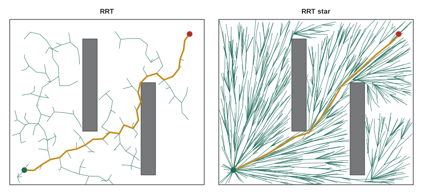
The key property is the Voronoi bias. A random sample is closest to a tree node with a probability equal to the volume of that node's Voronoi region, the set of points closer to it than to any other node. Nodes on the frontier of the tree, next to large unexplored areas, have large Voronoi regions and are extended most often; nodes deep inside explored areas have small regions and are rarely chosen. The tree therefore grows preferentially into unexplored space, rapidly spreading out to cover free space and then filling it in. RRT is probabilistically complete, but it is not optimal: Karaman and Frazzoli proved in 2011 that the cost of the RRT solution converges, with probability one, to a value that is in general strictly worse than optimal. The paths it finds are usually long and jagged, with random detours.
RRT-Connect
RRT-Connect (Kuffner and LaValle, 2000) grows two trees, one from the start and one from the goal. In each iteration one tree extends toward a random sample; then the other tree tries to connect to the newly added node by stepping repeatedly toward it until it either reaches it or hits an obstacle (the greedy 'connect' heuristic). The trees then swap roles. As soon as the two trees join, the path is complete. Bidirectional growth and greedy connection make RRT-Connect dramatically faster than a single RRT on most problems, often finding a path for a 7-joint arm in tens of milliseconds. Its paths are as jagged as RRT's, so they always need post-processing before execution.
import numpy as np
rng = np.random.default_rng(5)
OBS = [(3, 0, 4, 7), (6, 3, 7, 10)]               # rectangles (x0, y0, x1, y1) in a 10 x 10 space
def free(p): return not any(x0 <= p[0] <= x1 and y0 <= p[1] <= y1 for x0, y0, x1, y1 in OBS)
def seg_free(a, b):
    n = max(2, int(np.linalg.norm(b - a) / 0.05))
    return all(free(a + (b - a) * t) for t in np.linspace(0, 1, n))
def rrt(start, goal, eta=0.5, bias=0.05, iters=5000):
    nodes = [start]; parent = [-1]
    for it in range(iters):
        q = goal if rng.random() < bias else rng.uniform(0, 10, 2)
        i = int(np.argmin([np.linalg.norm(n - q) for n in nodes]))
        d = q - nodes[i]; dist = np.linalg.norm(d)
        new = q if dist <= eta else nodes[i] + eta * d / dist
        if seg_free(nodes[i], new):
            nodes.append(new); parent.append(i)
            if np.linalg.norm(new - goal) < 0.5 and seg_free(new, goal):
                nodes.append(goal); parent.append(len(nodes) - 2)
                k, L = len(nodes) - 1, 0.0
                while parent[k] >= 0: L += np.linalg.norm(nodes[k] - nodes[parent[k]]); k = parent[k]
                return it + 1, len(nodes), L
    return None
S, G = np.array([1.0, 1.0]), np.array([9.0, 9.0])
res = [rrt(S, G) for _ in range(10)]
res = [r for r in res if r]
print("solved %d of 10 runs" % len(res))
print("mean iterations %.0f, mean tree size %.0f" % (np.mean([r[0] for r in res]), np.mean([r[1] for r in res])))
print("mean path length %.2f (straight-line distance 11.31, shortest feasible about 19.1)" % np.mean([r[2] for r in res]))solved 10 of 10 runs mean iterations 542, mean tree size 328 mean path length 26.92 (straight-line distance 11.31, shortest feasible about 19.1)
RRT* and asymptotic optimality
RRT* (Karaman and Frazzoli, 2011) adds two steps to each extension. When \( q_{\text{new}} \) is created, instead of simply attaching it to \( q_{\text{near}} \), RRT* looks at all tree nodes within a radius r of \( q_{\text{new}} \) and chooses as its parent the one that gives the cheapest path from the start through a collision-free edge. Then it rewires: for each nearby node, if reaching it through \( q_{\text{new}} \) would be cheaper than its current path, its parent is changed to \( q_{\text{new}} \). With the radius shrinking as
for n nodes in d dimensions and a constant γ above a threshold that depends on the volume of free space, RRT* is asymptotically optimal: its solution cost converges to the optimum with probability one. The cost is more computation per iteration, since each new node triggers a radius search and several edge checks, roughly \( O(\log n) \) of them. Informed RRT* (Gammell, Srinivasa and Barfoot, 2014) speeds convergence once a first solution of cost \( c_{\text{best}} \) is known, by sampling only inside the ellipse of points whose straight-line distance to start plus goal is less than \( c_{\text{best}} \); no point outside it can improve the solution. Batch Informed Trees (BIT*) and related planners combine this with graph-search ordering and are among the best general-purpose asymptotically optimal planners available in OMPL.
Worked problem
Size of the informed sampling region
Start and goal are 8 m apart in a 2-D space of 20 m by 20 m. After RRT* finds a path of length 10 m, Informed RRT* samples only inside the ellipse with foci at start and goal whose points satisfy distance sum ≤ 10 m. What fraction of the space is that ellipse?
Show solution
- Semi-major axis: \( a = c_{\text{best}}/2 = 5 \) m.
- Half the focal distance: \( c = 4 \) m; semi-minor axis \( b = \sqrt{a^2 - c^2} = 3 \) m.
- Ellipse area: \( \pi a b = \pi \times 5 \times 3 = 47.1 \) m².
- Fraction: \( 47.1/400 = 0.118 \).
Answer: About 12 percent. Samples outside the ellipse cannot improve the path, so informed sampling makes every sample count, and the region shrinks further as the path improves.
Kinodynamic RRT
Steering a straight line toward a sample is fine for arms and holonomic robots, but a car cannot drive in a straight line to an arbitrary pose. Kinodynamic RRT replaces straight-line steering with simulation: from \( q_{\text{near}} \), apply a control input, chosen at random or from a small set of primitives, for a short time, integrate the robot's dynamics, and add the resulting state if the motion is collision-free. The tree then contains only feasible motions. The difficulty is that the nearest node under a simple metric may not be the easiest to extend toward the sample, and exactly reaching the goal state may be impossible without solving a boundary-value problem, so kinodynamic planners accept goal regions or use steering functions such as Dubins curves (lesson 10). Stable Sparse RRT (SST, Li, Littlefield and Bekris, 2016) extends kinodynamic planning with asymptotic near-optimality without needing a steering function.
Post-processing sampled paths
Raw sampled paths are never executed as they are. The standard pipeline first applies random shortcutting: repeatedly pick two points on the path at random and, if the straight segment between them is collision-free, replace the section between them. A few hundred attempts typically shorten an RRT-Connect path by 30 to 60 percent. Then the path is smoothed, for example by fitting splines through the remaining waypoints and checking the result, or by trajectory optimization (lesson 9). Finally it is time-parametrized respecting velocity and acceleration limits, as in ROB-300 lesson 8. In MoveIt 2 these steps are request adapters and post-processors that run automatically after the planner.
Worked problem
Is shortcutting worth it?
RRT-Connect returns a 3.8 rad joint-space path in 40 ms. Shortcutting with 200 attempts, each needing an average of 25 collision checks at 4 µs each, shortens the path to 2.1 rad. If the arm moves at 1.0 rad/s on average, does shortcutting pay for itself?
Show solution
- Shortcutting time: \( 200 \times 25 \times 4\,\mu s = 20 \) ms.
- Motion time saved: \( (3.8 - 2.1)/1.0 = 1.7 \) s.
- Net saving: about 1.68 s per move.
Answer: Yes: 20 ms of computation saves about 1.7 s of motion, and the shorter path is also less surprising to people nearby.
| Planner | Trees | Optimal? | Strength | Weakness |
|---|---|---|---|---|
| RRT | One from the start | No | Simple, explores quickly | Jagged, suboptimal paths |
| RRT-Connect | Two, greedy connection | No | Very fast for arms | Needs post-processing |
| RRT* | One, with rewiring | Asymptotically | Paths improve over time | Slower per iteration |
| Informed RRT* / BIT* | Focused after first solution | Asymptotically | Fast convergence | More complex |
| Kinodynamic RRT / SST | One, simulated controls | SST near-optimal | Respects dynamics | Hard to reach exact goals |
Common mistakes
MistakeExecuting a raw RRT path on a real arm
InsteadShortcut, smooth and time-parametrize it first.
MistakeUsing no goal bias, or a very large one
InsteadUse a small bias, around 5 to 10 percent, to pull toward the goal without losing exploration.
MistakeExpecting RRT paths to improve if the planner runs longer
InsteadPlain RRT is not asymptotically optimal; use RRT* or a variant.
MistakeUsing straight-line steering for a car-like robot
InsteadUse kinodynamic extension or Dubins/Reeds-Shepp steering.
MistakeKeeping the RRT* rewiring radius fixed and large
InsteadShrink it with log n / n so cost per iteration stays manageable.
Summary and key terms
- RRT grows a tree from the start toward random samples by steps of bounded size, stopping when it reaches the goal.
- The Voronoi bias makes frontier nodes extend most often, so the tree explores rapidly.
- RRT is probabilistically complete but not optimal, and its paths are jagged.
- RRT-Connect grows two trees with greedy connection and is among the fastest planners for arms.
- RRT* chooses the best parent and rewires neighbors within a shrinking radius, giving asymptotic optimality.
- Informed RRT* and BIT* focus sampling on the region that can still improve the solution.
- Kinodynamic RRT simulates controls; all sampled paths are shortcut, smoothed and time-parametrized before execution.
- RRT
- A rapidly-exploring random tree that grows toward random samples.
- Steering
- Extending a node toward a target configuration.
- Goal bias
- Sampling the goal itself with a small probability.
- Voronoi bias
- The tendency of RRT to extend nodes with large Voronoi regions.
- RRT-Connect
- A bidirectional RRT with greedy connection.
- RRT*
- An RRT variant with parent selection and rewiring that is asymptotically optimal.
- Rewiring
- Changing a node's parent to a newly added node when that is cheaper.
- Informed sampling
- Sampling only where a better solution could exist.
- Kinodynamic RRT
- An RRT that extends by simulating the robot's dynamics.
- Shortcutting
- Replacing sections of a path with straight collision-free segments.
Practice problems
Work each problem on paper first, then reveal the answer to check.
Node (0, 0), sample (3, 4), step 1: new node?
Show answer
(0.6, 0.8).
What does goal bias do?
Show answer
Samples the goal occasionally to pull the tree toward it.
Why do RRTs explore rapidly?
Show answer
Frontier nodes have large Voronoi regions and are extended most.
Is RRT asymptotically optimal?
Show answer
No.
How many trees does RRT-Connect grow?
Show answer
Two.
What two steps does RRT* add?
Show answer
Choosing the best parent and rewiring neighbors.
Ellipse semi-axes for start-goal distance 6 and best cost 10?
Show answer
a = 5, b = 4.
What does kinodynamic RRT do instead of straight-line steering?
Show answer
Simulates a control input on the dynamics.
Typical shortening from random shortcutting?
Show answer
About 30 to 60 percent.
Which RRT variant is MoveIt 2's usual default?
Show answer
RRT-Connect.
Lesson quiz · 5 questions
Score 60% or more to complete this lesson.
Create a free account to save your progress, take quizzes and earn a certificate.