
ROB-350 · Lesson 4 of 12 · 31 min
Graph search II: A* and heuristics
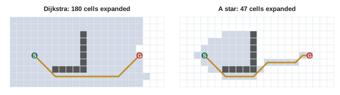
Dijkstra's algorithm spreads out evenly from the start, exploring cells behind the robot just as eagerly as cells toward the goal. When the goal's location is known, which in planning it always is, this wastes effort. The A* algorithm, introduced by Hart, Nilsson and Raphael in 1968 for the Shakey robot at the Stanford Research Institute, fixes this by adding an estimate of the remaining cost to each node's priority. With a good estimate, A* expands far fewer nodes than Dijkstra while still guaranteeing the cheapest path. It is the default search in grid and lattice planners, and the ideas behind it, heuristics, admissibility and consistency, run through the rest of planning.
This lesson explains how A* works and why it remains optimal, how to design heuristics for grids and lattices, and what happens when we deliberately trade optimality for speed with weighted A*. It then covers two refinements widely used on robots: Jump Point Search, which speeds up uniform grids, and incremental algorithms such as D* Lite, which repair a plan when the map changes instead of starting again.
The A* algorithm
A* orders the priority queue by \( f(n) = g(n) + h(n) \), where \( g(n) \) is the cost of the best known path from the start to n, as in Dijkstra, and \( h(n) \) is a heuristic estimate of the cost from n to the goal. Nodes that are cheap to reach and look close to the goal come out of the queue first. Everything else is the same as Dijkstra: pop the node with the smallest f, stop if it is the goal, otherwise relax its edges. With \( h = 0 \), A* is exactly Dijkstra. With a perfect heuristic, equal to the true remaining cost, A* expands only nodes on an optimal path. Real heuristics lie in between, and the better the heuristic, the fewer nodes are expanded.
Worked problem
Computing f values
On an 8-connected grid with unit cells, the goal is at (10, 4). Node A at (6, 4) has \( g = 7.0 \); node B at (3, 8) has \( g = 4.4 \). Using the octile heuristic \( h = \max(\Delta_x, \Delta_y) + (\sqrt{2} - 1)\min(\Delta_x, \Delta_y) \), which node does A* expand first?
Show solution
- A: \( \Delta_x = 4 \), \( \Delta_y = 0 \), so \( h = 4 \) and \( f = 11.0 \).
- B: \( \Delta_x = 7 \), \( \Delta_y = 4 \), so \( h = 7 + 0.414 \times 4 = 8.66 \) and \( f = 13.06 \).
- A has the smaller f.
Answer: Node A is expanded first, even though B has the smaller g. Dijkstra, using g alone, would have expanded B first, spending effort on a node that is further from the goal.
Admissible and consistent heuristics
A* returns an optimal path if its heuristic is admissible, meaning it never overestimates the true remaining cost: \( h(n) \le h^*(n) \) for every node. The argument is simple. When the goal is popped with cost C, every node still in the queue has \( f \ge C \), and since f underestimates the cost of any path through that node, no unexplored path can be cheaper than C. A stronger property, consistency (or monotonicity), requires that for every edge from n to n′, \( h(n) \le c(n, n') + h(n') \): the estimate cannot drop by more than the cost of a step. Consistent heuristics are admissible, and they guarantee that each node's g is final when it is first popped, so A* never needs to reopen a node. Almost all heuristics used in practice are consistent.
The standard heuristics are distances that ignore obstacles. On a 4-connected grid, the Manhattan distance \( |\Delta_x| + |\Delta_y| \) is exact in open space and admissible. On an 8-connected grid, the octile distance in the example above is exact in open space. Euclidean distance is admissible on any grid but underestimates on 4- and 8-connected grids, so A* expands more nodes than it needs to. For a car-like robot that must turn, Euclidean distance is a weak heuristic, and lattice planners use better ones, such as the length of the shortest Dubins or Reeds-Shepp curve ignoring obstacles (lesson 10), or a precomputed 2-D Dijkstra distance that accounts for obstacles but not turning. The maximum of two admissible heuristics is also admissible, which lets planners combine them.
| Heuristic | Formula | Admissible on | Notes |
|---|---|---|---|
| Zero | 0 | Any graph | A* becomes Dijkstra |
| Manhattan | |Δx| + |Δy| | 4-connected grids | Overestimates with diagonal moves |
| Octile | max + (√2 − 1)·min | 8-connected grids | Exact in open space |
| Euclidean | √(Δx² + Δy²) | Any metric graph | Weaker on grids, so more expansions |
| Dubins / Reeds-Shepp length | Shortest feasible curve, no obstacles | Car-like lattices | Accounts for turning |
| 2-D Dijkstra distance | Precomputed cost-to-go ignoring heading | (x, y, θ) lattices | Accounts for obstacles |
Worked problem
An inadmissible heuristic
A planner on an 8-connected grid mistakenly uses the Manhattan distance. The goal is 5 cells right and 5 cells up of a node in open space. What is the true cost, what does the heuristic say, and what can go wrong?
Show solution
- True cost with diagonals: \( 5\sqrt{2} \approx 7.07 \).
- Manhattan estimate: 10.
- The heuristic overestimates by 41 percent, so it is not admissible.
- A* may then pop the goal through a path that is not optimal, because a cheaper route looked too expensive and stayed in the queue.
Answer: The heuristic says 10 where the truth is 7.07. A* runs faster but can return a suboptimal path, typically one that avoids diagonals.
How much A* saves
The saving depends on how well the heuristic reflects the real cost. In open space with an exact heuristic, A* expands roughly the cells on a single straight corridor to the goal, compared with a disc of cells for Dijkstra. Obstacles reduce the saving: when a wall lies between the start and the goal, the heuristic is fooled into exploring the pocket in front of the wall until its f values rise to the true cost of going around. These 'heuristic depressions' are the main weakness of A*, and cost maps with many high-cost regions make them worse, because the heuristic, which assumes the minimum cost per cell, underestimates badly in expensive areas.
import heapq, math
grid = ["....................",
        "....................",
        "........#...........",
        "........#...........",
        "..S.....#........G..",
        "........#...........",
        "........#...........",
        "....................",
        "...................."]
R, C = len(grid), len(grid[0])
S = (4, 2); G = (4, 17)
moves = [(dr, dc, math.hypot(dr, dc)) for dr in (-1, 0, 1) for dc in (-1, 0, 1) if dr or dc]
def octile(n):
    dx, dy = abs(n[1] - G[1]), abs(n[0] - G[0])
    return max(dx, dy) + (math.sqrt(2) - 1) * min(dx, dy)
def search(w):                      # w = 0: Dijkstra; w = 1: A*; w > 1: weighted A*
    g = {S: 0.0}; pq = [(w * octile(S), S)]; done = set()
    while pq:
        f, u = heapq.heappop(pq)
        if u in done: continue
        done.add(u)
        if u == G: return g[u], len(done)
        for dr, dc, c in moves:
            v = (u[0] + dr, u[1] + dc)
            if 0 <= v[0] < R and 0 <= v[1] < C and grid[v[0]][v[1]] != "#" and g[u] + c < g.get(v, 1e9):
                g[v] = g[u] + c; heapq.heappush(pq, (g[v] + w * octile(v), v))
for name, w in (("Dijkstra", 0), ("A*", 1), ("weighted A*, w=2", 2)):
    cost, n = search(w)
print("%-17s cost %.3f expanded %3d" % (name, cost, n))Dijkstra cost 17.485 expanded 159 A* cost 17.485 expanded 60 weighted A*, w=2 cost 17.485 expanded 22
Weighted A* and anytime search
Multiplying the heuristic by a weight \( w > 1 \), so that \( f = g + w\,h \), makes A* greedier: it trusts the heuristic more and expands fewer nodes. The price is optimality, but in a controlled way. If h is admissible, the path found by weighted A* costs at most w times the optimal cost. A weight of 1.5 to 3 often cuts expansions by an order of magnitude in large maps while returning paths within a few percent of optimal in practice. Anytime planners exploit this: Anytime Repairing A* (ARA*, Likhachev, Gordon and Thrun, 2003) first plans quickly with a large weight, then lowers the weight and improves the path, reusing previous work, until time runs out. A robot can start moving on the first path and switch to better ones as they arrive.
Worked problem
The weighted A* bound
The optimal path in a warehouse map costs 84 m. A planner uses weighted A* with \( w = 1.8 \) and an admissible heuristic. What is the worst-case cost of the returned path? If ARA* then lowers w to 1.2, what is the new bound?
Show solution
- Bound: \( w \times C^* = 1.8 \times 84 = 151.2 \) m.
- With \( w = 1.2 \): \( 1.2 \times 84 = 100.8 \) m.
- In practice the first path is usually much closer to optimal than the bound.
Answer: At most 151 m at first, then at most 101 m. The bound guarantees the planner never returns anything absurd, while the robot gets a usable path quickly.
Jump Point Search
On a uniform-cost grid, many equal-cost paths differ only in the order of their horizontal and diagonal moves, and A* wastes time expanding all of them. Jump Point Search (Harabor and Grastien, 2011) prunes these symmetries. From each node it 'jumps' in a straight line, horizontally, vertically or diagonally, skipping over cells until it reaches a jump point: a cell where a forced neighbor appears because an obstacle ends, or the goal itself. Only jump points are placed in the queue. JPS returns optimal paths on uniform 8-connected grids and is often ten times faster than A* there. It does not apply directly to grids with varying costs, which limits its use on cost maps with inflation gradients.
Replanning: D* and D* Lite
Robots discover obstacles as they move: a pallet left in an aisle, a door that is closed. Replanning from scratch each time works but wastes the previous search. Incremental search algorithms repair it instead. Stentz's D* (1994), developed for outdoor vehicles at Carnegie Mellon and later used in Mars rover research, and Koenig and Likhachev's simpler D* Lite (2002) search backward from the goal, so that the robot's changing position does not invalidate the search tree. When edge costs change, only the nodes whose costs are affected are updated and re-expanded. D* Lite keeps two values per node, g and a one-step lookahead rhs, and processes nodes whose values disagree. When a new obstacle appears near the robot, only a small region needs repair; when it appears near the goal, more of the tree changes, and the saving over replanning from scratch is smaller.
Modern mobile robots often simply replan from scratch at a few hertz, because maps are small and A* is fast. Incremental methods remain valuable for large outdoor maps, for lattice planners where each expansion is expensive, and for robots exploring unknown terrain where the map changes continually.
Worked problem
When to replan
A global planner takes 40 ms for a full A* search on a 400 by 400 grid. The cost map updates at 5 Hz, and an incremental repair after a typical local change takes 6 ms. What fraction of one processor core does each approach use if the planner runs after every map update?
Show solution
- Full replanning: \( 5 \times 40 = 200 \) ms per second, 20 percent of a core.
- Incremental: \( 5 \times 6 = 30 \) ms per second, 3 percent of a core.
- Both fit within one core.
Answer: 20 percent versus 3 percent. On this map either approach works, which is why many systems use simple replanning; on a map ten times larger, the full search would take about a whole core and incremental repair would matter.
Common mistakes
MistakeUsing the Manhattan heuristic on an 8-connected grid
InsteadIt overestimates diagonal paths; use the octile distance.
MistakeAdding cost-map penalties without adjusting expectations of A*'s speed
InsteadThe heuristic underestimates in high-cost areas, so expansions grow; consider weighted A* or better heuristics.
MistakeAssuming weighted A* paths are optimal
InsteadThey are within w times optimal; state the bound.
MistakeApplying Jump Point Search to a grid with varying cell costs
InsteadJPS assumes uniform costs; use A* on cost maps.
MistakeRunning D* Lite from start to goal
InsteadIt searches backward from the goal so the robot's motion does not invalidate the tree.
Summary and key terms
- A* orders nodes by f = g + h, adding a heuristic estimate of remaining cost to Dijkstra's g.
- With an admissible heuristic, which never overestimates, A* returns an optimal path.
- Consistent heuristics also make each node final on its first expansion.
- Manhattan, octile and Euclidean distances suit different grids; car-like lattices need turning-aware heuristics.
- Weighted A* trades optimality for speed with a guaranteed bound of w times optimal; ARA* improves the path over time.
- Jump Point Search prunes symmetric paths on uniform grids.
- D* and D* Lite repair a backward search when edge costs change instead of replanning from scratch.
- A*
- Best-first search ordered by g + h.
- Heuristic
- An estimate of the remaining cost from a node to the goal.
- Admissible
- A heuristic that never overestimates the true remaining cost.
- Consistent
- A heuristic that drops by no more than the cost of each edge.
- Octile distance
- The exact open-space distance on an 8-connected grid.
- Heuristic depression
- A region where the heuristic underestimates badly, trapping the search.
- Weighted A*
- A* with an inflated heuristic, faster but bounded suboptimal.
- ARA*
- An anytime planner that lowers the heuristic weight over time.
- Jump Point Search
- A grid search that skips symmetric paths by jumping to key cells.
- D* Lite
- An incremental backward search that repairs plans when costs change.
Practice problems
Work each problem on paper first, then reveal the answer to check.
What is A* with h = 0?
Show answer
Dijkstra's algorithm.
Octile distance for Δx = 6, Δy = 2?
Show answer
6 + 0.414 × 2 ≈ 6.83.
What does admissibility guarantee?
Show answer
That A* returns an optimal path.
Is the Euclidean distance admissible on an 8-connected grid?
Show answer
Yes, but it underestimates, so A* expands more nodes.
Optimal cost 50, weight 2: worst-case weighted A* cost?
Show answer
100.
Why does a wall between start and goal slow A*?
Show answer
The heuristic underestimates and the search fills the pocket in front of the wall.
What kind of grid does Jump Point Search require?
Show answer
A uniform-cost grid.
Why does D* Lite search from the goal?
Show answer
So the robot's changing position does not invalidate the search.
Name a heuristic for a car-like robot.
Show answer
Dubins or Reeds-Shepp curve length.
Is the maximum of two admissible heuristics admissible?
Show answer
Yes.
Lesson quiz · 5 questions
Score 60% or more to complete this lesson.
Create a free account to save your progress, take quizzes and earn a certificate.