
ROB-350 · Lesson 6 of 12 · 28 min
Sampling-based planning I: probabilistic roadmaps
Grid search breaks down above three or four dimensions because the number of cells explodes. An arm with six or seven joints, a humanoid with thirty, or a mobile manipulator with ten degrees of freedom cannot be planned on a grid. Sampling-based planners avoid building the configuration space altogether. They pick configurations at random, ask a collision checker whether each is free, and connect nearby free configurations with short collision-free motions. The resulting graph captures the connectivity of free space without ever representing its boundary. This idea, developed in the mid-1990s, transformed motion planning: problems that had been intractable became solvable in seconds, and sampling-based planners are now the default for robot arms.
This lesson introduces the probabilistic roadmap (PRM), the first widely used sampling-based planner, published by Kavraki, Švestka, Latombe and Overmars in 1996. It covers how the roadmap is built and queried, what the collision checks along each edge involve, how the guarantees work, why narrow passages are the method's main weakness and how sampling strategies address them. Lesson 7 covers the tree-based planners, RRT and its variants, which are better suited to single queries.
The idea of a roadmap
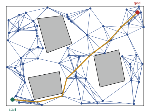
A PRM works in two phases. In the learning (construction) phase, it samples N configurations uniformly at random from C-space and keeps those that are collision-free as nodes. For each node, it then tries to connect it to nearby nodes, either its k nearest neighbors or all nodes within a radius r, using a local planner, usually a straight line in C-space. If every configuration along the line is free, the edge is added. In the query phase, the start and goal are connected to the roadmap in the same way, and a graph search (Dijkstra or A*, lessons 3 and 4) finds a path through it. Because the roadmap can be reused for many start-goal pairs in a static environment, PRM is called a multi-query planner. A robot arm working in a fixed cell, picking from the same bins all day, is the classic case.
Local planning and edge checking
Checking an edge means checking the continuous motion between two configurations, not just its endpoints. The usual method samples configurations along the segment at a resolution fine enough that no obstacle could fit between consecutive checks, then calls the collision checker for each. A common rule is to bound how far any point on the robot can move between checks. For an arm, the farthest-moving point is usually at the tool, and its displacement can be bounded from the joint changes and link lengths. Edge checking dominates the cost of PRM construction, so two tricks are standard. First, checking the midpoint first, then the quarter points, and so on (bisection order) finds collisions sooner on average than checking from one end. Second, lazy PRM (Bohlin and Kavraki, 2000) does not check edges during construction at all; it searches the unchecked roadmap, checks only the edges on the candidate path, removes any that collide and searches again. Since most edges are never on a candidate path, this saves much of the work.
Worked problem
How many checks along an edge?
A 6-joint arm moves between two configurations whose largest joint change is 0.6 rad. The farthest point on the arm is 1.1 m from the base, so it moves at most about 1.1 m per radian of joint motion. Obstacles are modeled with a 2 cm safety margin. How many intermediate configurations must be checked so that no point moves more than 2 cm between checks?
Show solution
- Maximum displacement of any point: about \( 1.1 \times 0.6 = 0.66 \) m (a conservative bound).
- Number of intervals: \( 0.66 / 0.02 = 33 \).
- So check 33 intermediate configurations plus the endpoints.
Answer: About 33 checks. A roadmap with 5,000 edges therefore needs on the order of 165,000 collision checks, which is why lazy evaluation pays off.
Nearest neighbors
Connecting each sample requires finding its nearest neighbors under the C-space metric of lesson 2, with angles wrapped and rotation weighted against translation. A brute-force search over N nodes costs \( O(N) \) per query and \( O(N^2) \) overall, which becomes significant for large roadmaps. Spatial data structures such as k-d trees, or approximate methods such as the geometric near-neighbor access tree used in OMPL, reduce this to roughly logarithmic time per query. The choice between k-nearest and radius connection also affects the guarantees. Karaman and Frazzoli showed in 2011 that connecting each node to its k nearest neighbors with k growing as a constant times \( \log N \), or within a radius shrinking as \( (\log N / N)^{1/d} \) in d dimensions, makes the roadmap asymptotically optimal; this variant is called PRM*. With a fixed k, PRM finds paths but their quality does not converge to the optimum.
Worked problem
Choosing k for PRM*
For a 6-dimensional C-space, what value of k does the PRM* rule give for N = 1,000 and N = 100,000 samples, using \( k_{\text{PRM}} = e(1 + 1/d) \) rounded up?
Show solution
- \( k_{\text{PRM}} = 2.718 \times (1 + 1/6) = 3.17 \).
- N = 1,000: \( 3.17 \times \ln 1000 = 3.17 \times 6.91 = 21.9 \), so k = 22.
- N = 100,000: \( 3.17 \times \ln 100{,}000 = 3.17 \times 11.51 = 36.5 \), so k = 37.
Answer: About 22 and 37 neighbors. The connection count grows only logarithmically, so a hundredfold larger roadmap needs fewer than twice as many connections per node.
Probabilistic completeness
PRM cannot prove that no path exists, but if one does, the probability of failing to find it decays exponentially with the number of samples. The rate depends on how 'open' free space is. Kavraki and colleagues formalized this with ε-goodness and expansiveness: if every free configuration can see at least a fraction ε of free space, then the probability that a roadmap of N samples fails to connect two points in the same component falls roughly like \( e^{-\epsilon N} \) times a factor depending on the path. In open environments ε is large and a few hundred samples suffice; in cluttered ones with narrow corridors, ε is tiny and the required N grows accordingly.
import numpy as np, heapq
rng = np.random.default_rng(1)
# 2-D C-space [0,10] x [0,10]; a wall at x in [4.5, 5.5] with a gap of width w around y = 5
def free(p, w):
    x, y = p
    return not (4.5 <= x <= 5.5 and abs(y - 5) > w / 2)
def edge_free(a, b, w, step=0.05):
    n = int(np.ceil(np.linalg.norm(b - a) / step))
    return all(free(a + (b - a) * t, w) for t in np.linspace(0, 1, n + 1))
def prm(N, w, k=10):
    pts = [np.array([1.0, 5.0]), np.array([9.0, 5.0])]
    while len(pts) < N + 2:
        p = rng.uniform(0, 10, 2)
        if free(p, w): pts.append(p)
    P = np.array(pts); adj = {i: [] for i in range(len(P))}
    for i in range(len(P)):
        d = np.linalg.norm(P - P[i], axis=1)
        for j in np.argsort(d)[1:k + 1]:
            if edge_free(P[i], P[j], w): adj[i].append(j); adj[j].append(i)
    seen = {0}; stack = [0]
    while stack:
        u = stack.pop()
        for v in adj[u]:
            if v not in seen: seen.add(v); stack.append(v)
    return 1 in seen
for w in (2.0, 0.5, 0.2):
    for N in (100, 400):
        ok = sum(prm(N, w) for _ in range(20))
print("gap %.1f, %3d samples: path found in %2d of 20 runs" % (w, N, ok))gap 2.0, 100 samples: path found in 18 of 20 runs gap 2.0, 400 samples: path found in 20 of 20 runs gap 0.5, 100 samples: path found in 8 of 20 runs gap 0.5, 400 samples: path found in 15 of 20 runs gap 0.2, 100 samples: path found in 2 of 20 runs gap 0.2, 400 samples: path found in 6 of 20 runs
Narrow passages
The narrow passage problem is the main weakness of uniform sampling. A corridor whose volume is a tiny fraction of C-space receives proportionally few samples, so the roadmap may fail to connect the regions it joins even when both sides are densely sampled. In high dimensions the effect is severe: a passage that is 1 percent of the width of each of six joint ranges occupies \( 10^{-12} \) of the volume in the worst case. Many sampling strategies concentrate samples where they help. Obstacle-based sampling (OBPRM) places samples near obstacle surfaces. Gaussian sampling draws pairs of points a short distance apart and keeps one only when the other is in collision, which puts samples near boundaries. The bridge test draws pairs whose endpoints are both in collision and keeps the free midpoint, which lands samples precisely inside narrow passages. Medial-axis sampling pushes samples toward the middle of free space for clearance. Each strategy improves performance on some problems and wastes effort on others, so planners often mix uniform sampling with one or more biased strategies.
Worked problem
Sample fraction in a narrow passage
In a 2-D C-space of 10 m by 10 m, a passage is 0.2 m wide and 1 m long. What fraction of uniform samples land in it, and how many samples on average are needed to place 5 inside it?
Show solution
- Passage area: \( 0.2 \times 1 = 0.2 \) m². C-space area: 100 m².
- Fraction: \( 0.2/100 = 0.002 \).
- Samples for 5 inside on average: \( 5/0.002 = 2{,}500 \).
Answer: Only 0.2 percent of samples land there, so about 2,500 samples are needed for five passage samples. A bridge test that keeps midpoints of pairs straddling the wall would place many more there.
| Strategy | How it samples | Helps with | Cost |
|---|---|---|---|
| Uniform | Uniformly over C-space | Open spaces | Few samples in narrow passages |
| Obstacle-based (OBPRM) | Near obstacle surfaces | Cluttered spaces | Extra collision checks to find surfaces |
| Gaussian | Pairs a short distance apart, one colliding | Regions near boundaries | Many rejected pairs |
| Bridge test | Midpoint of a colliding pair | Narrow passages | Very many rejections in open space |
| Medial axis | Pushed to the middle of free space | Clearance | Expensive retraction step |
| Lazy PRM | Uniform, edges checked only on demand | Expensive collision checks | Repeated searches |
When to use PRM
PRM shines when the environment is static and many queries will be made, because the roadmap amortizes its construction cost. It parallelizes easily, since samples and edges can be checked independently, and its roadmap can be stored and reused. For a single query in an environment that changes between queries, building a roadmap is wasteful, and the tree-based planners of lesson 7, which grow only toward the goal, are faster. Many arm planners in practice, including those in MoveIt 2 through OMPL, default to tree-based planners for this reason, while PRM and its variants remain the choice for repeated tasks in fixed work cells.
Common mistakes
MistakeChecking only the endpoints of roadmap edges
InsteadCheck the continuous motion at a resolution that bounds how far any point moves between checks.
MistakeUsing a Euclidean metric on joint angles that wrap around
InsteadWrap angular differences and weight joints sensibly.
MistakeExpecting PRM to report that no path exists
InsteadPRM is only probabilistically complete; failure may just mean too few samples.
MistakeRelying on uniform sampling in a cluttered cell with narrow gaps
InsteadAdd obstacle-based, Gaussian or bridge-test samples.
MistakeRebuilding a roadmap for every query in a static cell
InsteadPRM is multi-query; build once and reuse.
Summary and key terms
- Sampling-based planners sample free configurations and connect them, avoiding an explicit C-space.
- PRM builds a roadmap of free samples joined by collision-free local paths, then searches it for each query.
- Edge checking samples the motion finely enough to bound displacement between checks; lazy PRM defers it.
- Nearest-neighbor structures make connection fast; PRM* connects to k proportional to log N for asymptotic optimality.
- PRM is probabilistically complete, with failure probability decaying exponentially in the number of samples.
- Narrow passages receive few uniform samples; obstacle-based, Gaussian and bridge-test sampling address this.
- PRM suits static, multi-query settings; tree-based planners suit single queries.
- Probabilistic roadmap
- A graph of random free configurations joined by collision-free local paths.
- Multi-query planner
- A planner whose data structure is reused for many start-goal pairs.
- Local planner
- A simple method, often a straight line, for connecting two nearby configurations.
- Edge checking
- Testing a continuous motion for collisions by sampling along it.
- Lazy PRM
- A roadmap whose edges are checked only when they lie on a candidate path.
- PRM*
- A roadmap variant with log-growing connections that is asymptotically optimal.
- k-d tree
- A spatial data structure for fast nearest-neighbor queries.
- Narrow passage
- A small region of free space that connects larger regions.
- Bridge test
- Sampling the midpoint of two colliding configurations to find narrow passages.
- Expansiveness
- A measure of how easily free space can be covered by visible regions.
Practice problems
Work each problem on paper first, then reveal the answer to check.
What are the two phases of PRM?
Show answer
Construction (learning) and query.
Why is PRM called multi-query?
Show answer
The roadmap is reused for many start-goal pairs.
What does lazy PRM defer?
Show answer
Collision checking of edges.
Why check the midpoint of an edge first?
Show answer
It finds collisions sooner on average.
What k does PRM* use?
Show answer
A constant times log N.
What does probabilistic completeness promise?
Show answer
The chance of finding an existing path tends to one as samples increase.
Fraction of samples in a 0.5 m² passage of a 50 m² C-space?
Show answer
1 percent.
Which strategy keeps the free midpoint of two colliding samples?
Show answer
The bridge test.
Name one data structure for nearest neighbors.
Show answer
A k-d tree.
When is PRM a poor choice?
Show answer
For single queries in changing environments.
Lesson quiz · 5 questions
Score 60% or more to complete this lesson.
Create a free account to save your progress, take quizzes and earn a certificate.