
ROB-350 · Lesson 2 of 12 · 29 min
Configuration space
The single most useful idea in motion planning is to stop thinking about the robot as a shape moving among shapes and to think of it instead as a point moving through a space of configurations. This space, the configuration space or C-space, was introduced to robotics by Tomás Lozano-Pérez in 1979 and 1983. Each point in it is one complete placement of the robot. Some points correspond to placements where the robot overlaps an obstacle; together these form the C-space obstacle. The rest is free space. Planning a motion for a complicated robot among complicated obstacles becomes planning a path for a point through free space, and every search method in later lessons works on this formulation.
This lesson builds C-space step by step: for a point robot, for a disc, for a polygon that can rotate, and for a two-link arm. It shows how obstacles in the workspace map into C-space, introduces the Minkowski sum that makes this mapping exact for translating robots, discusses the shape and topology of C-space, and closes with the exact planning methods, visibility graphs and cell decompositions, that work directly on a polygonal free space.
Workspace and configuration space
The workspace is the physical space the robot moves in, usually the plane \( \mathbb{R}^2 \) or three-dimensional space \( \mathbb{R}^3 \). The configuration space is the set of all configurations q. For a robot whose configuration is n numbers, C-space has dimension n. A point robot in the plane has C-space equal to the plane itself, so its C-space obstacles are just the workspace obstacles. As soon as the robot has size or shape, the two spaces differ, and the difference is what makes C-space useful.
Formally, if \( A(q) \) is the set of workspace points occupied by the robot at configuration q and \( \mathcal{O} \) is the set of obstacle points, the C-space obstacle and free space are
A collision-free path is a continuous curve \( \tau : [0, 1] \to \mathcal{C}_{\text{free}} \) with \( \tau(0) = q_{\text{start}} \) and \( \tau(1) = q_{\text{goal}} \). Planners rarely compute \( \mathcal{C}_{\text{obs}} \) explicitly in high dimensions; instead they ask a collision checker, configuration by configuration, whether \( q \) is free. But understanding its shape explains why some problems are easy and others hard.
Discs and inflation
For a disc-shaped robot of radius r that translates without caring about orientation, the C-space obstacle is the workspace obstacle grown by r in every direction. A wall becomes a thicker wall; a square pillar becomes a square with rounded corners. This is the familiar 'inflation' step in mobile robot cost maps: every occupied cell is surrounded by a band of cells marked as untouchable, and the robot's center is then planned as a point. Inflation is exact for a disc. For a robot that is not round, using the radius of its circumscribed circle is conservative (it never allows a collision) but may block gaps the robot could actually fit through sideways; using the inscribed radius is optimistic and may allow collisions. Practical mobile planners therefore inflate by the inscribed radius to forbid certain collisions and check the full footprint only for poses near obstacles.
Worked problem
Inflating for a rectangular robot
A warehouse robot is 0.8 m long and 0.6 m wide. What are its inscribed and circumscribed radii, and can it pass, in any orientation, through a 0.9 m wide aisle and a 0.7 m wide gap?
Show solution
- Inscribed radius: half the shorter side, \( 0.6/2 = 0.30 \) m.
- Circumscribed radius: half the diagonal, \( \tfrac{1}{2}\sqrt{0.8^2 + 0.6^2} = 0.50 \) m.
- The 0.9 m aisle is narrower than the circumscribed diameter of 1.0 m, so the robot cannot rotate freely in it, but it can drive along it lengthwise because its width 0.6 m is less than 0.9 m.
- The 0.7 m gap is wider than the robot's width, so it fits only when aligned with the gap.
Answer: Inscribed 0.30 m, circumscribed 0.50 m. Both passages are traversable only with the right heading, so a planner that inflates by 0.50 m would wrongly declare both blocked. Orientation matters, and C-space must include θ.
Minkowski sums
For a robot that translates without rotating, there is an exact construction. Place a reference point on the robot and let \( -A \) be the robot's shape reflected through that point. Then the C-space obstacle of an obstacle \( \mathcal{O} \) is the Minkowski sum
Intuitively, slide the reflected robot around the boundary of the obstacle, keeping it touching; the reference point traces the boundary of the C-space obstacle. For convex polygons the sum is itself a convex polygon whose edges are the edges of both shapes sorted by angle, so it can be computed in time proportional to the total number of vertices. A square robot of side s moving among square obstacles of side d produces square C-obstacles of side \( s + d \). Non-convex shapes are handled by splitting them into convex pieces and taking the union of the pairwise sums.
Worked problem
A Minkowski sum by hand
A square robot of side 1 m has its reference point at its center. An obstacle occupies the rectangle from (3, 1) to (5, 2) m. What is the C-space obstacle?
Show solution
- The reflected robot is the same square, centered on the reference point, extending 0.5 m each way.
- The Minkowski sum of an axis-aligned rectangle and a square of half-width 0.5 m extends the rectangle by 0.5 m on every side.
- Lower-left corner: (3 − 0.5, 1 − 0.5) = (2.5, 0.5). Upper-right corner: (5 + 0.5, 2 + 0.5) = (5.5, 2.5).
Answer: The rectangle from (2.5, 0.5) to (5.5, 2.5) m. The robot's center must stay outside it. If the robot could rotate, the C-obstacle would change with θ and become a three-dimensional shape.
Rotation adds a dimension
When the robot can rotate, its configuration is \( (x, y, \theta) \) and C-space is three-dimensional. For each fixed heading θ, the slice of the C-obstacle is the Minkowski sum for the robot rotated to θ. Stacking these slices gives a twisted solid. A long, thin robot produces C-obstacles that are long in the direction perpendicular to its length for one heading and short for another, which is exactly why it can pass through a narrow gap when it is aligned with the gap. The heading dimension also wraps around: θ = 0 and θ = 2π are the same configuration, so C-space for a planar rigid body is not a box but \( \mathbb{R}^2 \times S^1 \), a plane times a circle.
Arms add their own geometry. A two-link planar arm with joint angles \( (\theta_1, \theta_2) \) has a C-space in which each angle wraps around, so it is a torus \( S^1 \times S^1 \) if the joints rotate fully, or a rectangle if joint limits stop them. A workspace obstacle produces a C-obstacle that can look nothing like it: a small block beside the arm may become a large curved band in the \( (\theta_1, \theta_2) \) plane, because many combinations of angles bring some part of the arm into contact. The figure shows such a mapping.
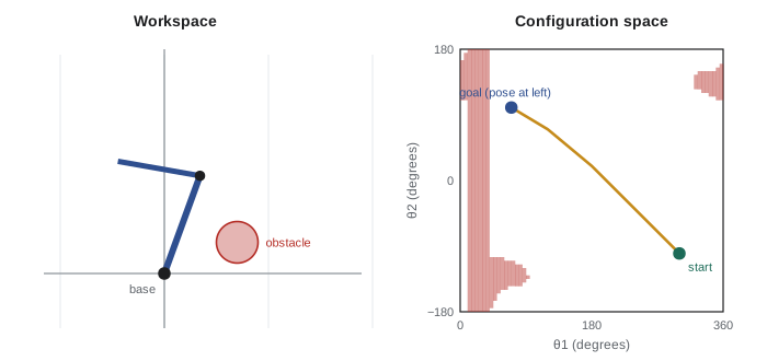
import numpy as np
# Two-link planar arm, links 1.0 m and 0.8 m; obstacle is a disc at (0.7, 0.3) radius 0.2, close to the base
L1, L2, ox, oy, R = 1.0, 0.8, 0.7, 0.3, 0.2
def seg_dist(ax, ay, bx, by):
    vx, vy = bx - ax, by - ay
    t = np.clip(((ox - ax) * vx + (oy - ay) * vy) / (vx * vx + vy * vy), 0, 1)
    return np.hypot(ax + t * vx - ox, ay + t * vy - oy)
n = 180                                   # 2-degree steps
th = np.radians(np.arange(n) * 2.0)
blocked = 0
for a in th:
    ex, ey = L1 * np.cos(a), L1 * np.sin(a)
    d1 = seg_dist(0, 0, ex, ey)
    for b in th - np.pi:
        fx, fy = ex + L2 * np.cos(a + b), ey + L2 * np.sin(a + b)
        if d1 < R or seg_dist(ex, ey, fx, fy) < R:
            blocked += 1
print("C-space cells:", n * n)
print("cells in collision: %d (%.1f %% of C-space)" % (blocked, 100 * blocked / n / n))
print("obstacle area / reachable workspace area: %.1f %%" % (100 * np.pi * R**2 / (np.pi * (L1 + L2)**2)))C-space cells: 32400 cells in collision: 3849 (11.9 % of C-space) obstacle area / reachable workspace area: 1.2 %
Topology and connectivity
Free space may be split into separate connected components. If the start and goal lie in different components, no path exists, however clever the planner. Determining connectivity is exactly what complete planners do; resolution-complete and sampling planners approximate it. The topology of C-space also creates traps for naive planners. Because θ wraps around, the shortest rotation from 350° to 10° is 20°, not 340°, and a planner that treats θ as an ordinary interval will produce wasteful spins. Distances on C-space must respect this wrap-around: for headings, use the angular difference wrapped into \( (-\pi, \pi] \); for arms with full-rotation joints, do the same per joint. Mixed spaces also need a weighting between translation and rotation, since one meter and one radian are not comparable without a choice of scale, often the robot's radius.
Worked problem
Distance in a wrapped space
Two configurations of a mobile robot are \( q_1 = (1.0, 2.0, 350^{\circ}) \) and \( q_2 = (1.6, 2.8, 20^{\circ}) \). Using the metric \( d = \sqrt{\Delta x^2 + \Delta y^2 + (\rho\,\Delta\theta)^2} \) with \( \rho = 0.4 \) m per radian, what is the distance?
Show solution
- Translation: \( \Delta x = 0.6 \), \( \Delta y = 0.8 \), so \( \sqrt{0.36 + 0.64} = 1.0 \) m.
- Wrapped heading difference: \( 20^{\circ} - 350^{\circ} = -330^{\circ} \), wrapped to \( +30^{\circ} = 0.524 \) rad.
- Weighted: \( 0.4 \times 0.524 = 0.209 \) m.
- \( d = \sqrt{1.0^2 + 0.209^2} \approx 1.02 \) m.
Answer: About 1.02 m. Without wrapping, the heading term would be \( 0.4 \times 5.76 = 2.30 \) m and the distance 2.5 m, badly misleading any planner that uses it to choose neighbors.
Exact methods in the plane
For a point (or inflated disc) robot among polygonal obstacles, the shortest path is made of straight segments between obstacle vertices. A visibility graph joins every pair of vertices, plus the start and goal, that can see each other without crossing an obstacle; the shortest path in this graph, found with Dijkstra's algorithm, is the true shortest path. It touches obstacles at their corners, which is optimal but unsafe for a real robot, so it is usually computed on obstacles inflated beyond the robot's size. Cell decomposition takes a different approach: split free space into simple cells, such as trapezoids by sweeping a vertical line across the obstacles' vertices, build a graph of adjacent cells, and search it. A generalized Voronoi diagram, the set of points equidistant from the two nearest obstacles, gives paths that maximize clearance and is the basis of some safe navigation methods. All three are exact and complete for polygonal problems in the plane, and all three are rarely used beyond it.
| Method | Path found | Strength | Limitation |
|---|---|---|---|
| Visibility graph | Shortest; grazes obstacle corners | Optimal and exact | Unsafe without inflation; 2-D polygons only |
| Trapezoidal decomposition | Through cell midpoints | Complete, simple to build | Paths not short; 2-D only |
| Generalized Voronoi diagram | Maximum clearance | Safe, few nodes | Long detours in open space |
| Grid search (lesson 5) | Near-shortest at the grid resolution | Works with sensor maps | Resolution complete only |
| Sampling (lessons 6 and 7) | Feasible, often jagged | Scales to many dimensions | Probabilistic guarantees only |
Common mistakes
MistakePlanning the robot's center as a point without inflating obstacles
InsteadInflate by the robot's radius, or check the full footprint, so the center path keeps the body clear.
MistakeInflating a rectangular robot by its circumscribed radius everywhere
InsteadThis blocks gaps the robot fits through when aligned; include heading or check the footprint near obstacles.
MistakeTreating heading as an ordinary interval from 0 to 2π
InsteadWrap angle differences so 350° to 10° is a 20° turn.
MistakeExpecting C-obstacles to look like workspace obstacles
InsteadFor arms and rotating robots, C-obstacles can be large, curved and disconnected.
MistakeFollowing a visibility-graph path on uninflated obstacles
InsteadThe path grazes corners; inflate first or add clearance.
Summary and key terms
- Configuration space represents every placement of the robot as a point; planning becomes moving a point through free space.
- For a translating disc, C-obstacles are workspace obstacles inflated by the radius.
- For a translating polygon, C-obstacles are Minkowski sums of the obstacle and the reflected robot.
- Rotation adds a dimension; heading wraps around, so planar C-space is a plane times a circle.
- Arm C-obstacles can be large, curved and unlike the workspace obstacles that cause them.
- Distances in C-space must wrap angles and weight rotation against translation.
- Visibility graphs, cell decompositions and Voronoi diagrams solve planar polygonal problems exactly.
- Configuration space
- The set of all configurations of a robot.
- C-space obstacle
- Configurations where the robot overlaps an obstacle.
- Free space
- Configurations where the robot touches no obstacle.
- Workspace
- The physical space the robot moves in.
- Minkowski sum
- The set of all sums of a point from one set and a point from another.
- Inflation
- Growing obstacles by the robot's radius so it can be planned as a point.
- Inscribed radius
- Radius of the largest circle that fits inside the robot's footprint.
- Circumscribed radius
- Radius of the smallest circle that contains the footprint.
- Visibility graph
- A graph joining mutually visible obstacle vertices, used for shortest paths.
- Generalized Voronoi diagram
- Points equidistant from the two nearest obstacles.
Practice problems
Work each problem on paper first, then reveal the answer to check.
What is C-space for a point robot in the plane?
Show answer
The plane itself.
A disc robot of radius 0.25 m: how much are obstacles inflated?
Show answer
0.25 m.
What shape is the Minkowski sum of two convex polygons?
Show answer
A convex polygon.
What is the topology of C-space for a planar rigid body?
Show answer
\( \mathbb{R}^2 \times S^1 \).
What is the topology for a two-link arm with unlimited joints?
Show answer
A torus.
Wrap a heading difference of 300°.
Show answer
−60°.
Inscribed radius of a 1.0 m by 0.5 m robot?
Show answer
0.25 m.
Which exact method gives maximum-clearance paths?
Show answer
The generalized Voronoi diagram.
Why is a visibility-graph path unsafe on raw obstacles?
Show answer
It touches obstacle corners.
What happens if start and goal are in different free-space components?
Show answer
No path exists.
Lesson quiz · 5 questions
Score 60% or more to complete this lesson.
Create a free account to save your progress, take quizzes and earn a certificate.