
ROB-350 · Lesson 9 of 12 · 32 min
Trajectory optimization
Search and sampling find a path that works; trajectory optimization finds one that is good. Instead of exploring a graph, an optimizer starts from an initial trajectory, often a straight line or the output of a sampling planner, and repeatedly adjusts it to reduce a cost that rewards smoothness and penalizes closeness to obstacles, subject to constraints such as joint limits and the start and goal. The results are the smooth, natural-looking motions that people expect from robots, and the same machinery extends to dynamics, torque limits and task constraints that search methods handle poorly. The price is locality: an optimizer improves the trajectory it is given and can get stuck in a local minimum, for example on the wrong side of an obstacle. Practical systems therefore combine optimization with search, using one to find the right homotopy class and the other to refine within it.
This lesson formulates trajectory optimization, builds the standard smoothness and obstacle costs, works through gradient descent on a simple path, and then surveys the influential methods: CHOMP, STOMP, TrajOpt and model predictive approaches. ROB-300 lesson 8 covered time scaling of a given path; here the shape of the path itself is the variable.
Formulating the problem
Discretize the trajectory into N waypoints \( \xi = (q_1, \ldots, q_N) \) between a fixed start \( q_0 \) and goal \( q_{N+1} \), equally spaced in time. The optimization problem is
where \( \mathcal{F}_{\text{smooth}} \) measures how much the trajectory bends or accelerates, \( \mathcal{F}_{\text{obs}} \) measures how close it comes to obstacles, and λ weights the two. Additional constraints can enforce velocity and acceleration limits, keep a held cup upright, or require the end effector to stay on a line. With N waypoints in a d-dimensional configuration space, the decision variable has \( N d \) entries, a few hundred for a typical arm trajectory, small enough for gradient-based methods to run in tens of milliseconds.
Smoothness costs
The simplest smoothness cost is the sum of squared differences between consecutive waypoints, a discrete version of the integral of squared velocity:
Because it is quadratic, its gradient is linear, \( A\xi + b \), where A is a tridiagonal finite-difference matrix with 2 on the diagonal and −1 beside it. Minimizing it alone gives evenly spaced waypoints on a straight line between start and goal. Penalizing squared accelerations, using second differences, gives smoother curves and is preferred for arms because it reduces jerky changes of speed; its matrix is pentadiagonal. Either way the smoothness cost is convex and well understood, and the difficulty lies entirely in the obstacle term.
Worked problem
Smoothness gradient for one waypoint
In 1-D, a waypoint \( q_i = 2.0 \) sits between neighbors \( q_{i-1} = 1.0 \) and \( q_{i+1} = 2.4 \). What is the gradient of the velocity smoothness cost with respect to \( q_i \), and which way does a gradient step move it?
Show solution
- The terms involving \( q_i \) are \( \tfrac{1}{2}(q_i - q_{i-1})^2 + \tfrac{1}{2}(q_{i+1} - q_i)^2 \).
- Derivative: \( (q_i - q_{i-1}) - (q_{i+1} - q_i) = 2q_i - q_{i-1} - q_{i+1} = 4.0 - 1.0 - 2.4 = 0.6 \).
- A gradient step subtracts a multiple of 0.6, moving \( q_i \) down toward the midpoint 1.7 of its neighbors.
Answer: The gradient is 0.6, so the waypoint moves toward 1.7, the average of its neighbors. Smoothness pulls each waypoint toward the midpoint of its neighbors, straightening the trajectory.
Obstacle costs
The obstacle term uses the signed distance field of lesson 8. Represent the robot by a set of body points or spheres; for each waypoint and each point, look up the distance d to the nearest obstacle and apply a cost that is zero when d exceeds a safety distance ε and grows as d shrinks. CHOMP uses a smooth version of this hinge:
Its gradient points along the distance field's gradient, away from the nearest obstacle, and its magnitude grows as the point approaches or penetrates the obstacle. Summing over body points and waypoints, weighted by how fast each point is moving so that slow, lingering contact costs more than a brief graze, gives \( \mathcal{F}_{\text{obs}} \). For an arm, the gradient with respect to the joint angles comes from the point's position Jacobian: \( \nabla_q c = J^{\mathsf{T}} \nabla_x c \), the same transpose-Jacobian mapping from forces to torques seen in ROB-300.
Worked problem
Evaluating the obstacle cost
With safety distance \( \varepsilon = 0.20 \) m, what is the CHOMP obstacle cost for body points at distances 0.30 m, 0.10 m and −0.05 m from the nearest obstacle?
Show solution
- At 0.30 m: greater than ε, so cost 0.
- At 0.10 m: \( \tfrac{1}{2 \times 0.2}(0.10 - 0.20)^2 = 2.5 \times 0.01 = 0.025 \).
- At −0.05 m (inside): \( 0.05 + 0.10 = 0.15 \).
Answer: 0, 0.025 and 0.15. The cost rises smoothly through the safety band and linearly inside obstacles, so the gradient always pushes points outward.
Gradient descent on a path
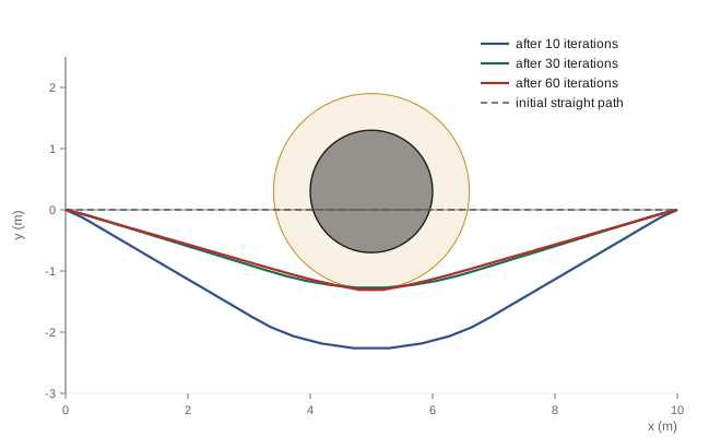
The simplest optimizer repeats \( \xi \gets \xi - \alpha \nabla \mathcal{U}(\xi) \) with a step size α, holding the start and goal fixed. Plain gradient descent works but converges slowly because the smoothness term is badly conditioned: moving one waypoint alone is cheap, while moving the whole trajectory together is what reduces the obstacle cost. CHOMP's key idea, covariant gradient descent, premultiplies the gradient by the inverse of the smoothness matrix, \( \xi \gets \xi - \tfrac{1}{\eta} A^{-1} \nabla \mathcal{U} \). This spreads each local correction smoothly along the whole trajectory, so a push away from an obstacle at one waypoint becomes a gentle bend over many, and convergence is dramatically faster. The code below runs this on a 2-D example.
import numpy as np
# 2-D path from (0, 0) to (10, 0) past a disc obstacle at (5, 0.3) radius 1.0; CHOMP-style covariant descent
N = 30; eps = 0.6; lam = 4.0
start, goal = np.array([0.0, 0.0]), np.array([10.0, 0.0])
xi = np.linspace(start, goal, N + 2)[1:-1].copy()        # straight line through the obstacle
xi[:, 1] += 0.05                                          # tiny nudge so the gradient picks a side
A = 2 * np.eye(N) - np.eye(N, k=1) - np.eye(N, k=-1)      # velocity finite differences
b = np.zeros((N, 2)); b[0] -= start; b[-1] -= goal
Ainv = np.linalg.inv(A)
c, R = np.array([5.0, 0.3]), 1.0
def obs(p):
    v = p - c; r = np.linalg.norm(v, axis=1, keepdims=True); d = r - R
    cost = np.where(d < 0, -d + eps / 2, np.where(d < eps, (d - eps) ** 2 / (2 * eps), 0))
    grad_d = np.where(d < 0, -1, np.where(d < eps, (d - eps) / eps, 0))
    return cost.sum(), grad_d * v / r
def clearance(p): return (np.linalg.norm(p - c, axis=1) - R).min()
def length(p):
    full = np.vstack([start, p, goal]); return np.linalg.norm(np.diff(full, axis=0), axis=1).sum()
print("iter  0: min clearance %+.2f m, length %.2f m" % (clearance(xi), length(xi)))
for it in range(1, 61):
    oc, og = obs(xi)
    grad = (A @ xi + b) + lam * og
    xi -= 0.03 * Ainv @ grad
    if it in (10, 30, 60):
print("iter %2d: min clearance %+.2f m, length %.2f m" % (it, clearance(xi), length(xi)))iter 0: min clearance -0.70 m, length 10.01 m iter 10: min clearance +1.58 m, length 11.12 m iter 30: min clearance +0.59 m, length 10.35 m iter 60: min clearance +0.62 m, length 10.35 m
Local minima and initialization
An optimizer only follows the gradient, so its result depends on where it starts. A straight-line initialization that passes exactly through the middle of an obstacle has a symmetric gradient and may stall, or be pushed to whichever side a small numerical asymmetry favors; one that starts on the far side of a wall cannot cross it. Each distinct way of going around obstacles is a homotopy class, and gradient methods stay within the class they start in. Practical remedies include restarting from several initial trajectories and keeping the best, initializing from a sampling planner's path, which is already in a feasible class, and adding random perturbations, as in CHOMP's Hamiltonian Monte Carlo variant. In MoveIt 2, CHOMP and STOMP are often run as post-processors on an OMPL path for exactly this reason.
Worked problem
Restarts and success rate
Experiments show that an optimizer started from a random initial trajectory reaches a collision-free solution 35 percent of the time on a cluttered task, and runs take 30 ms. How many independent restarts are needed for a 95 percent chance of success, and how long does that take?
Show solution
- Failure probability with k restarts: \( 0.65^k \).
- Require \( 0.65^k \le 0.05 \): \( k \ge \ln 0.05/\ln 0.65 = 2.996/0.431 = 6.95 \), so 7 restarts.
- Time: \( 7 \times 30 = 210 \) ms, less if run in parallel.
Answer: Seven restarts, about 210 ms sequentially. Seeding with an RRT-Connect path that is already feasible usually does better than random restarts.
CHOMP, STOMP and TrajOpt
CHOMP (Covariant Hamiltonian Optimization for Motion Planning; Ratliff, Zucker, Bagnell and Srinivasa, 2009) is the method sketched above: smoothness plus SDF-based obstacle cost, minimized by covariant gradient descent. STOMP (Stochastic Trajectory Optimization for Motion Planning; Kalakrishnan, Chitta, Theodorou, Pastor and Schaal, 2011) needs no gradients: it generates noisy variations of the current trajectory, evaluates their costs, and combines them weighted by how well they did. This lets it handle costs that are not differentiable, such as torque limits computed by simulation or discontinuous constraints. TrajOpt (Schulman and colleagues, 2013 and 2014) formulates the problem as sequential convex optimization: at each iteration it linearizes collision constraints using signed distances between convex shapes (computed by GJK and EPA), solves a convex quadratic program within a trust region, and repeats. Treating collision avoidance as a constraint rather than a penalty, and checking continuous swept volumes between waypoints, makes TrajOpt reliable at producing truly collision-free results.
| Method | Uses gradients? | Collision handling | Strength | Limitation |
|---|---|---|---|---|
| Gradient descent | Yes | Penalty from SDF | Simple | Slow, ill-conditioned |
| CHOMP | Yes, covariant | Penalty from SDF on body spheres | Fast, smooth results | Local minima; penalty not a guarantee |
| STOMP | No, sampled | Any cost | Handles non-smooth costs | More cost evaluations |
| TrajOpt | Yes, sequential convex | Linearized signed-distance constraints | Reliable collision-free output | More complex; needs convex shapes |
| MPC planners | Yes, receding horizon | Constraints over a short horizon | Reacts online | Short-sighted without a global plan |
Constraints and dynamics
Optimizers handle constraints naturally. Joint limits are bounds on the variables. Velocity and acceleration limits become constraints on finite differences of waypoints once the time step is fixed, or the time step itself can be a variable for time-optimal problems. Task constraints, such as keeping an end effector's orientation within 5° of vertical, become nonlinear equality or inequality constraints on forward kinematics. Including the full dynamics, \( M(q)\ddot{q} + C(q, \dot{q})\dot{q} + g(q) = \tau \) from ROB-300, with torque limits gives direct transcription and collocation methods, the basis of trajectory planning for legged robots and fast arms. Model predictive control applies the same optimization on a short, receding horizon at control rates, which lesson 11 uses for dynamic environments.
Worked problem
Velocity limits as constraints
A trajectory for one joint has waypoints every 0.05 s. The joint's velocity limit is 2.0 rad/s. What constraint does this place on consecutive waypoints, and is the step from 0.42 rad to 0.55 rad allowed?
Show solution
- Velocity estimate: \( (q_{i+1} - q_i)/\Delta t \).
- Constraint: \( |q_{i+1} - q_i| \le 2.0 \times 0.05 = 0.10 \) rad.
- Step: \( 0.55 - 0.42 = 0.13 \) rad, which exceeds 0.10 rad.
Answer: Each step must be at most 0.10 rad, so the 0.13 rad step violates the limit. The optimizer must spread the motion over more time or more waypoints.
Common mistakes
MistakeInitializing the optimizer with a straight line through obstacles and trusting the result
InsteadSeed it with a feasible sampled path or run restarts.
MistakeTreating a low obstacle penalty as proof of no collisions
InsteadValidate the final trajectory with an exact collision checker, including between waypoints.
MistakeUsing plain gradient descent with a fixed small step
InsteadPrecondition with the smoothness metric, as in CHOMP, or use a proper solver.
MistakeIgnoring joint and velocity limits during optimization
InsteadInclude them as bounds or constraints rather than clipping afterwards.
MistakeChoosing the obstacle weight once and never tuning it
InsteadToo low allows grazing; too high distorts paths. Tune λ and ε for the task.
Summary and key terms
- Trajectory optimization improves an initial trajectory by minimizing smoothness and obstacle costs subject to constraints.
- Velocity and acceleration smoothness costs are quadratic, with finite-difference matrices.
- Obstacle costs use a signed distance field over body points, with gradients mapped to joints by the Jacobian transpose.
- Covariant gradient descent spreads corrections along the whole trajectory and converges much faster than plain descent.
- Optimizers stay in the homotopy class they start in, so initialization and restarts matter.
- CHOMP, STOMP and TrajOpt differ in using gradients, sampling or sequential convex programming.
- Joint, velocity, task and dynamic constraints fit naturally into the optimization.
- Trajectory optimization
- Improving a trajectory by minimizing a cost subject to constraints.
- Waypoint
- One of the discrete configurations that represent a trajectory.
- Smoothness cost
- A cost penalizing velocity or acceleration along a trajectory.
- Obstacle cost
- A cost penalizing proximity to obstacles.
- Covariant gradient descent
- Gradient descent preconditioned by the smoothness metric.
- Homotopy class
- A family of paths that can be deformed into each other without crossing obstacles.
- CHOMP
- A gradient-based trajectory optimizer using signed distance fields.
- STOMP
- A sampling-based, gradient-free trajectory optimizer.
- TrajOpt
- Sequential convex trajectory optimization with signed-distance constraints.
- Direct transcription
- Optimizing states and controls at discrete times subject to the dynamics.
Practice problems
Work each problem on paper first, then reveal the answer to check.
What does minimizing the velocity smoothness cost alone produce?
Show answer
Evenly spaced waypoints on a straight line.
Gradient of the velocity cost at q = 3 with neighbors 2 and 3.6?
Show answer
2(3) − 2 − 3.6 = 0.4.
CHOMP cost at d = 0.05 m with ε = 0.25 m?
Show answer
(0.2)² / 0.5 = 0.08.
How is a Cartesian gradient mapped to joints?
Show answer
By the Jacobian transpose.
Why does covariant descent converge faster?
Show answer
It spreads each correction smoothly along the trajectory.
What limits gradient-based optimizers in cluttered scenes?
Show answer
Local minima within the starting homotopy class.
Which method needs no gradients?
Show answer
STOMP.
How does TrajOpt treat collisions?
Show answer
As linearized signed-distance constraints.
Velocity limit 1.5 rad/s, Δt 0.02 s: largest step?
Show answer
0.03 rad.
Name one way to avoid bad local minima.
Show answer
Seed from a sampling planner or use restarts.
Lesson quiz · 5 questions
Score 60% or more to complete this lesson.
Create a free account to save your progress, take quizzes and earn a certificate.